Incorporating linear models

In previous juliet tutorials for transits (Lightcurve fitting with juliet) and radial-velocities (Fitting radial-velocities), we have so far assumed that the only deterministic signals under consideration in the models \(\mathcal{M}_i(t)\) for instrument \(i\) are composed of underlying physical processes. For transits, we assume the function is a transit model distorted both by a normalization constant and a dilution factor, whereas for the radial-velocities we assume this is an addition between a Keplerian signal, a systemic radial-velocity and a long-term trend. Typically, however, these are not the only components that make up a model. For transits, systematics in the data (e.g., airmass trends, meridian flips, etc.) can distort the signals further — for radial-velocities some linear models might help out constrain activity signals.

Within juliet one can model, in addition to the deterministic signal for transits and radial-velocities, \(\mathcal{M}_i(t)\), a linear model such that the full data-generating process can be written as

\(\mathcal{M}_i(t) + \textrm{LM}_i(t) + \epsilon_i(t)\),

where the terms \(\mathcal{M}_i(t)\) is the transit or radial-velocity model, \(\epsilon_i(t)\) is the noise model (for details on those, see previous tutorials on transits and radial-velocities), and where \(\textrm{LM}_i(t)\) is a linear model given by:

\(\textrm{LM}_i(t) = \sum_{n=0}^{p_i}x_{n,i}(t) \theta_{n,i}^{\textrm{LM}}\).

Here, the \(x_{n,i}(t)\) are the \(p_i+1\) linear regressors at time \(t\) for instrument \(i\), and the \(\theta_{n,i}^{\textrm{LM}}\) are the coefficients of those regressors (e.g., \(x_{n,i}(t) = t^n\) would model a polynomial trend for instrument \(i\)).

Linear models in transit fits

Adding linear terms to a model within juliet is very simple, and can be done in two ways. One way is to simply pack the lightcurve and regressors in a text file of the form:

2458459.7999999998 1.0126748331 0.0030000000 CHAT 1.2107127967
2458459.8013377925 1.0127453892 0.0030000000 CHAT 1.2107915485
2458459.8026755853 1.0158682599 0.0030000000 CHAT 1.2108919775
2458459.8040133780 1.0117892069 0.0030000000 CHAT 1.2110140837
2458459.8053511707 1.0125201749 0.0030000000 CHAT 1.2111578671
2458459.8066889634 1.0133562197 0.0030000000 CHAT 1.2113233277
.
.
.

where, the first column saves the times, second the relative fluxes, third errors on these relative fluxes, fourth the instrument names and the \(p_i+1\) subsequent columns store the \(p_i+1\) linear regressors to be fitted to the data (in the above example, 1). Once this file is created, the filename can be simply given to the juliet.load call with the lcfilename parameter — this will store the times, lightcurves and linear regressors in a given dataset. The second way is to simply pass all the linear regressors using the linear_regressors_lc variable of the juliet.load call — the input should be a dictionary, where each key is a different instrument and contains an array of dimensions \((N_i, p_i+1)\), where \(N_i\) is the number of datapoints for instrument \(i\). In this tutorial, we will use the former way of fitting linear models.

In this tutorial we will use the dataset uploaded [here] — this dataset has one linear regressor. For each linear regressor, we must define the prior for the coefficient \(\theta_{n,i}\); these are expected to be of the form thetaN_i, where N is the numbering of the linear regressor (as given in the file or dictionary) and i is the instrument name. In our case, we have data from the CHAT telescope — let’s fit it assuming a linear model:

import juliet
import numpy as np

priors = {}

# Name of the parameters to be fit:
params = ['P_p1','t0_p1','r1_p1','r2_p1','q1_CHAT','q2_CHAT','ecc_p1','omega_p1',\
              'rho', 'mdilution_CHAT', 'mflux_CHAT', 'sigma_w_CHAT', 'theta0_CHAT']

# Distributions:
dists = ['fixed','normal','uniform','uniform','uniform','uniform','fixed','fixed',\
                 'loguniform', 'fixed', 'normal', 'loguniform', 'uniform']

# Hyperparameters
hyperps = [3.1, [2458460,0.1], [0.,1], [0.,1.], [0., 1.], [0., 1.], 0.0, 90.,\
                   [100., 10000.], 1.0, [0.,0.1], [0.1, 1000.],[-100,100]]

# Populate the priors dictionary:
for param, dist, hyperp in zip(params, dists, hyperps):
    priors[param] = {}
    priors[param]['distribution'], priors[param]['hyperparameters'] = dist, hyperp


# Load dataset:
dataset = juliet.load(priors=priors, lcfilename = 'lc_lm.dat', out_folder = 'lm_transit_fit')
results = dataset.fit(n_live_points = 300)

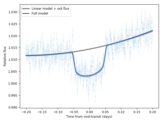
Now let’s plot it:

t0 = np.median(results.posteriors['posterior_samples']['t0_p1'])

# Plot. First extract model:
transit_model, transit_up68, transit_low68, components  = results.lc.evaluate('CHAT', return_err=True, \
                                                                              return_components = True, \
                                                                              all_samples = True)

import matplotlib.pyplot as plt
plt.errorbar(dataset.times_lc['CHAT']-t0, dataset.data_lc['CHAT'], \
             yerr = dataset.errors_lc['CHAT'], fmt = '.' , alpha = 0.1)

# Out-of-transit flux:
oot_flux = np.median(1./(1. + results.posteriors['posterior_samples']['mflux_CHAT']))

# Plot non-transit model::
plt.plot(dataset.times_lc['CHAT']-t0, oot_flux + components['lm'], color='grey', lw = 3, label = 'Linear model + oot flux')
plt.plot(dataset.times_lc['CHAT']-t0, transit_model, color='black', label = 'Full model')
plt.fill_between(dataset.times_lc['CHAT']-t0,transit_up68,transit_low68,\
                 color='cornflowerblue',alpha=0.5,zorder=5)

plt.xlabel('Time from mid-transit (days)')
plt.ylabel('Relative flux')
plt.legend()