Lightcurve fitting with juliet
We have already exemplified how to fit a basic transit lightcurve in the Getting started section with juliet. Here, however,
we explore some interesting extra features of the lightcurve fitting process, including limb-darkening laws, parameter transformations and
fitting of data from multiple-instruments simultaneously, along with useful details on the model evaluations with juliet.
Before going into the tutorial, it is useful to first understand the lightcurve model that juliet uses. In the absence of extra
linear terms (which we will deal with in the Incorporating linear models tutorial), a juliet lightcurve model for a given instrument
\(i\) is given by (see Section 2 of the juliet paper)
\(\mathcal{M}_{i}(t) + \epsilon_i(t)\),
where
\(\mathcal{M}_{i}(t) = [\mathcal{T}_{i}(t)D_{i} + (1-D_{i})]\left(\frac{1}{1+D_{i}M_{i}}\right)\)
is the photometric model composed of the dilution factor \(D_{i}\), the relative out-of-transit target flux \(M_{i}\), and the transit model for the instrument \(\mathcal{T}_{i}(t)\) (defined by the transit parameters and by the instrument-dependant limb-darkening coefficients — see the Models, priors and outputs section for details). Here, \(\epsilon_i(t)\) is a stochastic process that defines a “noise model” for the dataset. In this section we will assume that \(\epsilon_i(t)\) is white-gaussian noise, i.e., \(\epsilon_i(t)\sim \mathcal{N}(0,\sqrt{\sigma_i(t)^2 + \sigma_{w,i}^2})\), where \(\mathcal{N}(\mu,\sigma)\) denotes a normal distribution with mean \(\mu\) and standard-deviation \(\sigma\), and where \(\sigma_i(t)\) are the errors on the datapoint at time \(t\) and \(\sigma_{w,i}\) is a so-called “jitter” term. We deal with more general noise models in the Incorporating Gaussian Processes tutorial.
The juliet lightcurve model is a bit different than typical lightcurve models which typically only fit for an out-of-transit
flux offset. The first difference is that our model includes a dilution factor \(D_{i}\) which allows the user to account for possible contaminating
sources in the aperture that might produce a smaller transit depth than the real one. In fact, if there are \(n\) sources with
fluxes \(F_n\) in the aperture and the target has a flux \(F_T\), then one can show (see Section 2 of the
juliet paper) that the dilution factor can be interpreted as
\(D_i = \frac{1}{1 + \sum_n F_n/F_T}\).
A dilution factor of 1, thus, implies no external contaminating sources. The second difference is that the relative out-of-transit target flux, \(M_i\) — which from hereon we refer to as the “mean out-of-transit flux” — is a multiplicative term and not an additive offset. This is because input lightcurves are usually normalized (typically with respect to the mean or the median), and in theory a simple additive offset might thus still not account for this pre-normalization of the lightcurve. \(M_i\), in turn, has a well defined interpretation: if the real out-of-transit flux was \(F_T + \sum_n F_n + E\), where \(E\) is an offset flux given by light coming not from the sources \(F_n\) or from the target, \(F_T\) (e.g., background scattered light, a bias flux, etc.), then this term can be interpreted as \(E/F_T\). As can be seen, then, with \(D_i\) and \(M_i\), one can uniquely recover the real (relative to the target) fluxes.
Transit fits
To showcase the ability of juliet to fit transit lightcurves, we will play with the HATS-46b system
(Brahm et al., 2017), as the TESS data for this system has interesting features that
we will be using both in this tutorial and in the Incorporating Gaussian Processes tutorial. In this tutorial in particular, we will
play with the data obtained in Sector 2, because it seems the level of variability/systematics in this particular dataset
is much smaller than the one for Sector 1 (which we tackle in the Incorporating Gaussian Processes tutorial). First, let us download and plot the
TESS data, taking the opportunity to also put the data in dictionaries so we can feed it to juliet:
import juliet
import numpy as np
import matplotlib.pyplot as plt

# First, get arrays of times, normalized-fluxes and errors for HATS-46
# from Sector 1 from MAST:
t, f, ferr  = juliet.get_TESS_data('https://archive.stsci.edu/hlsps/'+\
                                   'tess-data-alerts/hlsp_tess-data-'+\
                                   'alerts_tess_phot_00281541555-s02_'+\
                                   'tess_v1_lc.fits')

# Put data arrays into dictionaries so we can fit it with juliet:
times, fluxes, fluxes_error = {},{},{}
times['TESS'], fluxes['TESS'], fluxes_error['TESS'] = t,f,ferr

# Plot data:
plt.errorbar(t, f, yerr=ferr, fmt='.')
plt.xlim([np.min(t),np.max(t)])

Pretty nice dataset! The transits can be clearly seen by eye. The period seems to be about \(P \sim 4.7\) days, in agreement with the Brahm et al., 2017 study, and the time-of-transit center seems to be about \(t_0 \sim 1358.4\) days. Let us now fit this lightcurve using these timing constraints as priors. We will use the same “non-informative” priors for the rest of the transit parameters as was already done for TOI-141b in the Getting started tutorial:
priors = {}

# Name of the parameters to be fit:
params = ['P_p1','t0_p1','r1_p1','r2_p1','q1_TESS','q2_TESS','ecc_p1','omega_p1',\
              'rho', 'mdilution_TESS', 'mflux_TESS', 'sigma_w_TESS']

# Distributions:
dists = ['normal','normal','uniform','uniform','uniform','uniform','fixed','fixed',\
                 'loguniform', 'fixed', 'normal', 'loguniform']

# Hyperparameters
hyperps = [[4.7,0.1], [1358.4,0.1], [0.,1], [0.,1.], [0., 1.], [0., 1.], 0.0, 90.,\
                   [100., 10000.], 1.0, [0.,0.1], [0.1, 1000.]]

# Populate the priors dictionary:
for param, dist, hyperp in zip(params, dists, hyperps):
    priors[param] = {}
    priors[param]['distribution'], priors[param]['hyperparameters'] = dist, hyperp
Now let’s fit the dataset with juliet, saving the results to a folder called hats46:
# Load and fit dataset with juliet:
dataset = juliet.load(priors=priors, t_lc = times, y_lc = fluxes, \
                   yerr_lc = fluxes_error, out_folder = 'hats46')

results = dataset.fit()
As was already shown in the Getting started tutorial, it is easy to plot the juliet fit results using the
results.lc.evaluate() function. In the background, this function extracts by default nsamples=1000 random
samples from the joint posterior distribution of the parameters and evaluates the model using them —
by default, a call to this function given an instrument name returns the median of all of those models. However, one can
also retrieve the models that are about “1-sigma away” from this median model — i.e., the 68% credibility band of these
models — by setting return_err=True. One can actually select the percentile credibility band with the alpha parameter
(by default, alpha=0.68). Let us extract and plot the median model and the corresponding 68% credibility band around it using
this function. We will create two plots: one of time versus flux, and another one with the phased transit lightcurve:
# Extract median model and the ones that cover the 68% credibility band around it:
transit_model, transit_up68, transit_low68  = results.lc.evaluate('TESS', return_err=True)

# To plot the phased lighcurve we need the median period and time-of-transit center:
P, t0 = np.median(results.posteriors['posterior_samples']['P_p1']),\
        np.median(results.posteriors['posterior_samples']['t0_p1'])

# Get phases:
phases = juliet.get_phases(dataset.times_lc['TESS'], P, t0)


import matplotlib.gridspec as gridspec

# Plot the data. First, time versus flux --- plot only the median model here:
fig = plt.figure(figsize=(12,4))
gs = gridspec.GridSpec(1, 2, width_ratios=[2,1])
ax1 = plt.subplot(gs[0])

ax1.errorbar(dataset.times_lc['TESS'], dataset.data_lc['TESS'], \
             yerr = dataset.errors_lc['TESS'], fmt = '.' , alpha = 0.1)

# Plot the median model:
ax1.plot(dataset.times_lc['TESS'], transit_model, color='black',zorder=10)

# Plot portion of the lightcurve, axes, etc.:
ax1.set_xlim([np.min(dataset.times_lc['TESS']),np.max(dataset.times_lc['TESS'])])
ax1.set_ylim([0.96,1.04])
ax1.set_xlabel('Time (BJD - 2457000)')
ax1.set_ylabel('Relative flux')

# Now plot phased model; plot the error band of the best-fit model here:
ax2 = plt.subplot(gs[1])
ax2.errorbar(phases, dataset.data_lc['TESS'], \
             yerr = dataset.errors_lc['TESS'], fmt = '.', alpha = 0.3)
idx = np.argsort(phases)
ax2.plot(phases[idx],transit_model[idx], color='black',zorder=10)
ax2.fill_between(phases[idx],transit_up68[idx],transit_low68[idx],\
                 color='white',alpha=0.5,zorder=5)
ax2.set_xlabel('Phases')
ax2.set_xlim([-0.015,0.015])
ax2.set_ylim([0.98,1.02])
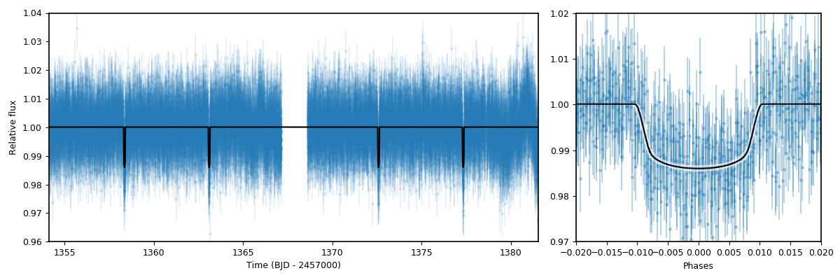
As can be seen, the lightcurve model is quite precise! In the code above we also made use of a function and a dictionary which we have not introduced in
their entirety yet. The first is the juliet.get_phases(t, P, t0) function — this gives you back the phases at the times t given a period P and
a time-of-transit center t0. The second is a very important dictionary: it was already briefly introduced in the Models, priors and outputs section, but
this introduction did not pay justice to its importance. This is the results.posteriors dictionary. The posterior_samples key of this dictionary
stores the posterior distribution of the fitted parameters — we make use of this dictionary in detail in the next part of the tutorial.
Transit parameter transformations
In the fit done in the previous section we fitted the Sector 2 TESS lightcurve of HATS-46b. There, however, we fitted for the transformed parameters
r1_p1 and r2_p1 which parametrize the planet-to-star radius ratio, \(p = R_p/R_*\), and the impact parameter, in our case given by
\(b = (a/R_*)\cos i\), and the limb-darkening parametrization q1_TESS and q2_TESS, which in our case parametrize the coefficients \(u_1\) and
\(u_2\) of the quadratic limb-darkening law. How do we transform the posterior distributions of those parametrizations, stored in the
results.posteriors['posterior_samples'] dictionary back to their physical parameters? juliet has built-in functions to do just this.
To transform from the \((r_1,r_2)\) plane to the \((b,p)\) plane, we have implemented the transformations described in
Espinoza (2018). These require one defines the minimum and maximum allowed
planet-to-star radius ratio — by default, within juliet the parametrization allows to
search for all planet-to-star radius ratios from \(p_l = 0\) to \(p_u = 1\) (and these can be modified in the fit object — e.g.,
dataset.fit(...,pl= 0.0, pu = 0.2)). The values used for each fit are always stored in results.posteriors['pl'] and results.posteriors['pu'].
In our case, then, to obtain the posterior distribution of \(b\) and \(p\), we can use the juliet.utils.reverse_bp(r1,r2,pl,pu) function which
takes samples from the \((r_1,r_2)\) plane and converts them back to the \((b,p)\) plane. Let us do this transformation for the HATS-46b fit done above
and compare with the results obtained in Brahm et al., 2017:
fig = plt.figure(figsize=(5,5))
# Store posterior samples for r1 and r2:
r1, r2 = results.posteriors['posterior_samples']['r1_p1'],\
         results.posteriors['posterior_samples']['r2_p1']

# Transform back to (b,p):
b,p = juliet.utils.reverse_bp(r1, r2, 0., 1.)

# Plot posterior distribution:
plt.plot(b,p,'.',alpha=0.5)

# Extract median and 1-sigma errors for b and p from
# the posterior distribution:
bm,bu,bl = juliet.utils.get_quantiles(b)
pm,pu,pl = juliet.utils.get_quantiles(p)

# Plot them:
plt.errorbar(np.array([bm]),np.array([pm]),\
             xerr = np.array([[bu-bm,bm-bl]]),\
             yerr = np.array([[pu-pm,pm-pl]]),\
             fmt = 'o', mfc = 'white', mec = 'black',\
             ecolor='black', ms = 15, elinewidth = 3, \
             zorder = 5, label = 'This work')

# Plot values in Brahm et al. (2017):
plt.errorbar(np.array([0.634]),np.array([0.1088]),\
             xerr = np.array([[0.042,0.034]]), \
             yerr = np.array([0.0027]),zorder = 5,\
             label = 'Brahm et al. (2017)', fmt='o', \
             mfc = 'white', elinewidth = 3, ms = 15)

plt.legend()
plt.xlim([0.,0.8])
plt.ylim([0.1,0.125])
plt.xlabel('$b$')
plt.ylabel('$p = R_p/R_*$')
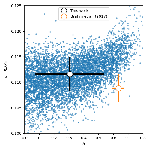
The agreement with Brahm et al., 2017 is pretty good! The planet-to-star radius ratios are consistent within one-sigma, and the (uncertain for TESS) impact parameter is consistent at less thant 2-sigma with the one published in that work.
What about the limb-darkening coefficients? juliet also has a built-in function to perform the inverse
transformation in order to obtain them — this is the juliet.utils.reverse_ld_coeffs() function — given
a limb-darkening law and the parameters \(q_1\) and \(q_2\), this function gives back the limb-darkening
coefficients \(u_1\) and \(u_2\). Let us plot the posterior distribution of the limb-darkening coefficients;
let’s compare them to theoretical limb-darkening coefficients using limb-darkening (Espinoza & Jordan, 2015):
fig = plt.figure(figsize=(5,5))
# Store posterior samples for q1 and q2:
q1, q2 = results.posteriors['posterior_samples']['q1_TESS'],\
          results.posteriors['posterior_samples']['q2_TESS']

# Transform back to (u1,u2):
u1, u2 = juliet.utils.reverse_ld_coeffs('quadratic', q1, q2)

# Plot posterior distribution:
plt.plot(u1,u2,'.',alpha=0.5)

# Plot medians and errors implied by the posterior:
u1m,u1u,u1l = juliet.utils.get_quantiles(u1)
u2m,u2u,u2l = juliet.utils.get_quantiles(u2)
plt.errorbar(np.array([u1m]),np.array([u2m]),\
             xerr = np.array([[u1u-u1m,u1m-u1l]]),\
             yerr = np.array([[u2u-u2m,u2m-u2l]]),\
             fmt = 'o', mfc = 'white', mec = 'black',\
             ecolor='black', ms = 13, elinewidth = 3, \
             zorder = 5, label = 'This work')

plt.plot(np.array([0.346,0.346]),np.array([-1,1]),'--',color='cornflowerblue')
plt.plot(np.array([-1,1]),np.array([0.251,0.251]),'--',color='cornflowerblue',label='ATLAS')

plt.plot(np.array([0.377,0.377]),np.array([-1,1]),'--',color='red')
plt.plot(np.array([-1,1]),np.array([0.214,0.214]),'--',color='red',label='PHOENIX')
plt.legend()

plt.xlabel('$u_1$')
plt.ylabel('$u_2$')
plt.xlim([0.0,1.0])
plt.ylim([-0.5,1.0])
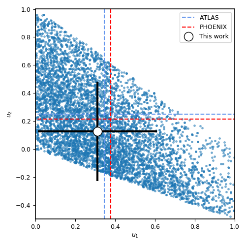
The agreement with the theory is pretty good in this case! It was kind of expected — HATS-46 is a solar-type star after all. Notice the triangular shape of the parameter spaced explored? This is what the \((q_1,q_2)\) sampling is expected to sample — the triangle englobes all the physically plausible parameter space for the limb-darkening coefficients (positive, decreasing-to-the-limb limb-darkening profiles). For details, see Kipping (2013).
Fitting multiple datasets
In the previous sections we have been fitting the TESS data only. What if we want to add extra datasets
and fit all of them jointly in order to extract the posterior distribution of the transit parameters? As
it was already mentioned, this is very easy to do with juliet: you simply add new elements/keys to the
dictionary one gives as inputs to it. Of course, you also have to add some extra priors for the extra
instruments: in particular, one has to define a jitter (\(\sigma_{w,i}\)), dilution factor (\(D_i\)),
mean out-of-transit flux (\(M_i\)) and limb-darkening parametrization (\(q_1\) if a linear law wants to be
assumed, or also give \(q_2\) if a quadratic law wants to be used). Let us fit the TESS data together with the follow-up
lightcurves obtained by Brahm et al., 2017 from the Las Cumbres Observatory Global
Telescope Network (LCOGT) and the 1m Swope Telescope. These can be obtained from CDS following the paper link, but we have
uploaded them here and
here so it is easier to follow this
tutorial. Once that data is downloaded, we can load this data in juliet as follows:
# Add LCOGT and SWOPE data to the times, fluxes and fluxes_error dictionary.
# Fill also the priors for these instruments:
for instrument in ['LCOGT','SWOPE']:
    # Open dataset files, extract times, fluxes and errors to arrays:
    t2,f2,ferr2 = np.loadtxt('hats-46_data_'+instrument+'.txt',\
                              unpack=True,usecols=(0,1,2))
    # Add them to the data dictionaries which already contain the TESS data (see above):
    times[instrument], fluxes[instrument], fluxes_error[instrument] = \
                                                t2-2457000, f2, ferr2

    # Add priors to the already defined ones above for TESS, but for the other instruments:
    params = ['sigma_w_','mflux_','mdilution_','q1_','q2_']
    dists = ['loguniform', 'normal', 'fixed', 'uniform', 'uniform']
    hyperps = [[0.1,1e5], [0.0,0.1], 1.0, [0.0,1.0], [0.0,1.0]]

    for param, dist, hyperp in zip(params, dists, hyperps):
        priors[param+instrument] = {}
        priors[param+instrument]['distribution'], \
        priors[param+instrument]['hyperparameters'] = dist, hyperp
And with this one can simply run a juliet fit again:
dataset = juliet.load(priors=priors, t_lc = times, y_lc = fluxes, \
                      yerr_lc = fluxes_error, out_folder = 'hats46-extra')

results = dataset.fit(n_live_points=300)
This can actually take a little bit longer than just fitting the TESS data (a couple of extra minutes) — it is a 17-dimensional problem after all. Let us plot the results of the joint instrument fit:
# Extract new period and time-of-transit center:
P,t0 =  np.median(results.posteriors['posterior_samples']['P_p1']),\
        np.median(results.posteriors['posterior_samples']['t0_p1'])

# Generate arrays to super-sample the models:
model_phases = np.linspace(-0.04,0.04,1000)
model_times = model_phases*P + t0

# Plot figure:
fig = plt.figure(figsize=(10,3))
instruments = ['TESS','LCOGT','SWOPE']
alphas = [0.1, 0.5, 0.5]
for i in range(3):
    instrument = instruments[i]
    plt.subplot('13'+str(i+1))
    # Plot phase-folded data:
    phases = juliet.utils.get_phases(dataset.times_lc[instrument], P, t0)
    plt.errorbar(phases, dataset.data_lc[instrument], \
                 yerr = dataset.errors_lc[instrument], fmt = '.' , alpha = alphas[i])
    # Evaluate model in the supersampled times, plot on top of data:
    model_lc = results.lc.evaluate(instrument, t = model_times)
    plt.plot(model_phases,model_lc,color='black')
    plt.title(instrument)
    plt.xlabel('Phase')
    if i == 0:
        plt.ylabel('Relative flux')
    plt.xlim([-0.025,0.025])
    plt.ylim([0.975,1.02])
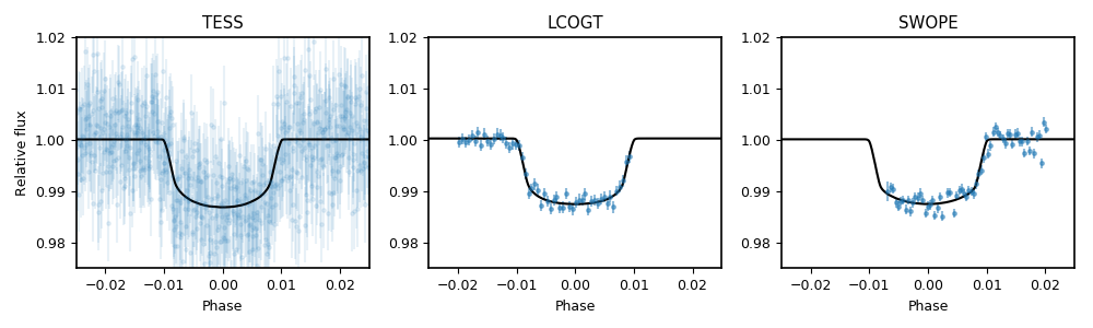
Pretty nice fit! The Swope data actually shows a little bit more scatter — indeed, the \(\sigma_{w,SWOPE} = 1269^{+185}_{-155}\) ppm, which indicates that there seems to be some extra process happening in the lightcurve (e.g., systematics), which are being modelled in our fit with a simple jitter term. So, how does the posteriors of our parameters compare with that of the TESS-only fit? We can repeat the plot made above for the planet-to-star radius ratio and impact parameter to check:
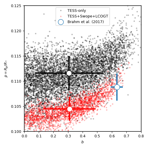
Interesting! The transit depth is consistent between fits and with the work of Brahm et al., 2017. Interestingly, the impact parameter is practically the same as the TESS-only fit, and just shrinked a little bit. It is still consistent at 2-sigma with the work of Brahm et al., 2017, however.
A word on limb-darkening and model selection
Throughout the tutorial, we have not explicitly defined what limb-darkening laws we wanted to use for each dataset. By default, juliet assumes that if the
user defines \(q_1\) and \(q_2\), then a quadratic law wants to be used, whereas if the user only gives \(q_1\), a linear-law is assumed.
In general, the limb-darkening law to use depends on the system under study (see, e.g.,
Espinoza & Jordan, 2016.), and thus the user might want to use laws other than the ones that
are pre-defined by juliet. This can be easily done when loading a dataset via juliet.load using the ld_laws flag. This flag receives a
string with the name of the law to use — currently supported laws are the linear, the quadratic, the logarithmic and the squareroot laws.
We don’t include the exponential law in this list as it has been shown to be a non-physical law in Espinoza & Jordan, 2016.
Let us test how the different laws do on the TESS dataset of HATS-46b. For this, let us fit the dataset with all the available limb-darkening laws and check the log-evidences, \(\ln \mathcal{Z} = \ln \mathcal{P}(D | \textrm{Model})\) each model gives. Assuming all the models are equally likely, the different log-evidences can be transformed to odds ratios (i.e., the ratio of the probabilities of the models given the data, \(\mathcal{P}(\textrm{Model}_i|D)/\mathcal{P}(\textrm{Model}_j|D)\)) by simply substracting the log-evidences of the different models, i.e.,
\(\ln \frac{\mathcal{P}(\textrm{Model}_i|D)}{\mathcal{P}(\textrm{Model}_j|D)} = \ln \frac{\mathcal{P}(D | \textrm{Model}_i)}{\mathcal{P}(D|\textrm{Model}_j)} = \ln \frac{Z_i}{Z_j}\),
if \(P(\textrm{Model}_i)/P(\textrm{Model}_j) = 1\). juliet also extracts the model evidences in the results.posteriors dictionary under the lnZ key; errors on this
log-evidence calculation are under lnZerr. Let us compute the log-evidences for each limb-darkening law and compare them to see which one is the “best” in terms of this
model comparison tool:
# Load Sector 1 data for HATS-46b again:
t, f, ferr  = juliet.get_TESS_data('https://archive.stsci.edu/hlsps/'+\
                                   'tess-data-alerts/hlsp_tess-data-'+\
                                   'alerts_tess_phot_00281541555-s02_'+\
                                   'tess_v1_lc.fits')

# Put data arrays into dictionaries so we can fit it with juliet:
times, fluxes, fluxes_error = {},{},{}
times['TESS'], fluxes['TESS'], fluxes_error['TESS'] = t,f,ferr

# Define limb-darkening laws to test:
ld_laws = ['linear','quadratic','logarithmic','squareroot']

for ld_law in ld_laws:
     priors = {}
     # If law is not the linear, set priors for q1 and q2. If linear, set only for q1:
     if ld_law != 'linear':
         params = ['P_p1','t0_p1','r1_p1','r2_p1','q1_TESS','q2_TESS','ecc_p1','omega_p1',\
                   'rho', 'mdilution_TESS', 'mflux_TESS', 'sigma_w_TESS']

         dists = ['normal','normal','uniform','uniform','uniform','uniform','fixed','fixed',\
                      'loguniform', 'fixed', 'normal', 'loguniform']

         hyperps = [[4.7,0.1], [1358.4,0.1], [0.,1], [0.,1.], [0., 1.], [0., 1.], 0.0, 90.,\
                        [100., 10000.], 1.0, [0.,0.1], [0.1, 1000.]]
     else:
         params = ['P_p1','t0_p1','r1_p1','r2_p1','q1_TESS','ecc_p1','omega_p1',\
                   'rho', 'mdilution_TESS', 'mflux_TESS', 'sigma_w_TESS']

         dists = ['normal','normal','uniform','uniform','uniform','fixed','fixed',\
                      'loguniform', 'fixed', 'normal', 'loguniform']

         hyperps = [[4.7,0.1], [1358.4,0.1], [0.,1], [0.,1.], [0., 1.], 0.0, 90.,\
                        [100., 10000.], 1.0, [0.,0.1], [0.1, 1000.]]

     for param, dist, hyperp in zip(params, dists, hyperps):
         priors[param] = {}
         priors[param]['distribution'], priors[param]['hyperparameters'] = dist, hyperp

     dataset = juliet.load(priors=priors, t_lc = times, y_lc = fluxes, \
                           yerr_lc = fluxes_error, out_folder = 'hats46-'+ld_law, \
                           ld_laws = ld_law)

     results = dataset.fit()
     print("lnZ for "+ld_law+" limb-darkening law is: ",results.posteriors['lnZ']\
                                               ,"+-",results.posteriors['lnZerr'])
In our runs this gave:
lnZ for linear limb-darkening law is:      64202.653 +- 0.040
lnZ for quadratic limb-darkening law is:   64202.182 +- 0.018
lnZ for logarithmic limb-darkening law is: 64202.652 +- 0.077
lnZ for squareroot limb-darkening law is:  64202.786 +- 0.041
At face value, the model with the largest log-evidence is the square-root law, whereas the one with the lowest log-evidence is the quadratic law. However, the difference between those two log-evidences is very small: only \(\Delta \ln Z = 0.60\) in favor of the square-root law, or an odds ratio between those laws of \(\exp\left(\Delta \ln Z\right) \approx 2\) — given the data, the square-root law model is only about two times more likely than the quadratic law. Not much, to be honest — I wouldn’t bet my money on the quadratic law being wrong, so our assumption of a quadratic limb-darkening law in our analyses above seems to be very good. It is unlikely more complex limb-darkening laws would have given better results, by the way: note how the simpler linear law is basically equally likely to the square-root law (\(\exp\left(\Delta \ln Z\right) \approx 1\)).
What if more than one instrument is being fit; how do we define limb-darkening laws for each instrument? The ld_laws flag can also take as input a comma-separated string where one indicates the law to be
used for each instrument in the form instrument-ldlaw. For example, if we wanted to fit the TESS, LCOGT and Swope data and define a square-root law for the former and logarithmic law for the other instruments,
we would do (assuming we have already loaded the data and priors to the priors, times, fluxes and fluxes_error dictionaries):
dataset = juliet.load(priors=priors, t_lc = times, y_lc = fluxes, \
                      yerr_lc = fluxes_error,\
                      ld_laws = 'TESS-squareroot,LCOGT-logarithmic,SWOPE-logarithmic')

results = dataset.fit()