Getting started
Two ways of using juliet
In the spirit of accomodating the code for everyone to use, juliet can be used in two different ways: as
an imported library and also in command line mode. Both give rise to the same results because the command
line mode simply calls the juliet libraries in a python script.
To use juliet as an imported library, inside any python script you can simply do:
import juliet
dataset = juliet.load(priors = priors, t_lc=times, y_lc=flux, yerr_lc=flux_error)
results = dataset.fit()
In this example, juliet will perform a fit on a lightcurve dataset defined by a dictionary of times times,
relative fluxes flux and error on those fluxes flux_error given some prior information priors which,
as we will see below, is also defined through a dictionary.
In command line mode, juliet can be used through a simple call in any terminal. To do this, after
installing juliet, you can from anywhere in your system simply do:
juliet -flag1 -flag2 --flag3
In this example, juliet is performing a fit using different inputs defined by -flag1, -flag2 and --flag3.
There are several flags that can be used to accomodate your juliet runs through command-line which we’ll explore
in the tutorials. There is a third way of using juliet, which is by calling the juliet.py code and applying
these same flags (as it is currently explained in project’s wiki page).
However, no further updates will be done for that method, and the ones defined above should be the preferred ones to
use.
A first fit to data with juliet
To showcase how juliet works, let us first perform an extremely simple fit to data using juliet as an imported library.
We will fit the TESS data of TOI-141 b, which was shown to host a 1-day transiting exoplanet by
Espinoza et al. (2019). Let us first load the data corresponding to this
object, which is hosted in MAST. For TESS data, juliet has already built-in functions to load the data arrays
directly given a web link to the data — let’s load it and plot the data to see how it looks:
import juliet
import numpy as np
# First, get times, normalized-fluxes and errors for TOI-141 from MAST:
t,f,ferr  = juliet.get_TESS_data('https://archive.stsci.edu/hlsps/tess-data-alerts/'+\
                                 'hlsp_tess-data-alerts_tess_phot_00403224672-'+\
                                 's01_tess_v1_lc.fits')

# Plot the data!
import matplotlib.pyplot as plt
plt.errorbar(t,f,yerr=ferr,fmt='.')

plt.xlim([np.min(t),np.max(t)])
plt.ylim([0.999,1.001])
plt.xlabel('Time (BJD - 2457000)')
plt.ylabel('Relative flux')

This will save arrays of times, fluxes (PDCSAP_FLUX fluxes, in particular) and errors on the t, f and ferr arrays. Now,
in order to load this dataset into a format that juliet likes, we need to put these into dictionaries. This, as we will
see, will make it extremely easy to add data from more instruments, as these will be simply stored in different
keys of the same dictionary. For now, let us just use this TESS data; we put them in dictionaries that juliet likes as
follows:
# Create dictionaries:
times, fluxes, fluxes_error = {},{},{}
# Save data into those dictionaries:
times['TESS'], fluxes['TESS'], fluxes_error['TESS'] = t,f,ferr
# If you had data from other instruments you would simply do, e.g.,
# times['K2'], fluxes['K2'], fluxes_error['K2'] = t_k2,f_k2,ferr_k2
The final step to fit the data with juliet is to define the priors for the different parameters that we
are going to fit. This can be done in two ways. The longest (but more jupyter-notebook-friendly?) is to
create a dictionary that, on each key, has the names of the parameter to be fitted. Each of those elements
will be dictionaries themselves, containing the distribution of the parameter and their corresponding
hyperparameters (for details on what distributions juliet can handle, what are the hyperparameters and
what each parameter name mean, see the next section of this document: Models, priors and outputs).
Let us give normal priors for the period P_p1, time-of-transit center t0_p1, mean out-of-transit
flux mflux_TESS, uniform distributions for the parameters r1_p1 and r2_p1 of the
Espinoza (2018) parametrization
for the impact parameter and planet-to-star radius ratio, same for the q1_p1 and q2_p1
Kipping (2013)
limb-darkening parametrization (juliet assumes a quadratic limb-darkening by default — other laws can
be easily defined, as it will be shown in the tutorials), log-uniform distributions for the stellar density
rho (in kg/m3) and jitter term sigma_w_TESS (in parts-per-million, ppm), and leave the rest of the
parameters (eccentricity ecc_p1, argument of periastron (in degrees) omega_p1 and dilution factor
mdilution_TESS) fixed:
priors = {}

# Name of the parameters to be fit:
params = ['P_p1','t0_p1','r1_p1','r2_p1','q1_TESS','q2_TESS','ecc_p1','omega_p1',\
              'rho', 'mdilution_TESS', 'mflux_TESS', 'sigma_w_TESS']

# Distribution for each of the parameters:
dists = ['normal','normal','uniform','uniform','uniform','uniform','fixed','fixed',\
                 'loguniform', 'fixed', 'normal', 'loguniform']

# Hyperparameters of the distributions (mean and standard-deviation for normal
# distributions, lower and upper limits for uniform and loguniform distributions, and
# fixed values for fixed "distributions", which assume the parameter is fixed)
hyperps = [[1.,0.1], [1325.55,0.1], [0.,1], [0.,1.], [0., 1.], [0., 1.], 0.0, 90.,\
                   [100., 10000.], 1.0, [0.,0.1], [0.1, 1000.]]

# Populate the priors dictionary:
for param, dist, hyperp in zip(params, dists, hyperps):
    priors[param] = {}
    priors[param]['distribution'], priors[param]['hyperparameters'] = dist, hyperp
With these definitions, to fit this dataset with juliet one would simply do:
# Load dataset into juliet, save results to a temporary folder called toi141_fit:
dataset = juliet.load(priors=priors, t_lc = times, y_lc = fluxes, \
                      yerr_lc = fluxes_error, out_folder = 'toi141_fit')

# Fit and absorb results into a juliet.fit object:
results = dataset.fit(n_live_points = 300)
This code will run juliet and save the results both to the results object and to the toi141_fit
folder.
The second way to define the priors for juliet (and perhaps the most simple) is to create a text file where
in the first column one defines the parameter name, in the second column the name of the distribution and
in the third column the hyperparameters. The priors defined above would look like this in a text file:
P_p1                 normal               1.0,0.1
t0_p1                normal               1325.55,0.1
r1_p1                uniform              0.0,1.0
r2_p1                uniform              0.0,1.0
q1_TESS              uniform              0.0,1.0
q2_TESS              uniform              0.0,1.0
ecc_p1               fixed                0.0
omega_p1             fixed                90.0
rho                  loguniform           100.0,10000.0
mdilution_TESS       fixed                1.0
mflux_TESS           normal               0.0,0.1
sigma_w_TESS         loguniform           0.1,1000.0
To run the same fit as above, suppose this prior file is saved under toi141_fit/priors.dat. Then, to load this
dataset into juliet and fit it, one would do:
# Load dataset into juliet, save results to a temporary folder called toi141_fit:
dataset = juliet.load(priors='toi141_fit/priors.dat', t_lc = times, y_lc = fluxes, \
                      yerr_lc = fluxes_error, out_folder = 'toi141_fit')

# Fit and absorb results into a juliet.fit object:
results = dataset.fit(n_live_points = 300)
And that’s it! Cool juliet fact is that, once you have defined an out_folder, all your data will be saved there —
not only the prior file and the results of the fit, but also the photometry or radial-velocity you fed into juliet will
be saved. This makes it easy to come back later to this dataset without having to download the data all over again, or
re-run your fits. So, for example, suppose we have already ran the code above, closed our terminals, and wanted to come back
at this dataset again with another python session and say, plot the data and best-fit model. To do this one can simply do:
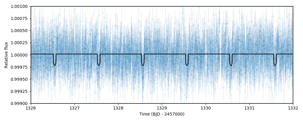
import juliet

# Load already saved dataset with juliet:
dataset = juliet.load(input_folder = 'toi141_fit', out_folder = 'toi141_fit')

# Load results (the data.fit call will recognize the juliet output files in
# the toi141_fit folder generated when we ran the code for the first time):
results = dataset.fit()

import matplotlib.pyplot as plt

# Plot the data:
plt.errorbar(dataset.times_lc['TESS'], dataset.data_lc['TESS'], \
             yerr = dataset.errors_lc['TESS'], fmt = '.', alpha = 0.1)

# Plot the model:
plt.plot(dataset.times_lc['TESS'], results.lc.evaluate('TESS'))

# Plot portion of the lightcurve, axes, etc.:
plt.xlim([1326,1332])
plt.ylim([0.999,1.001])
plt.xlabel('Time (BJD - 2457000)')
plt.ylabel('Relative flux')
plt.show()
Which will give us a nice plot of the data and the juliet fit:
Warning
When using MultiNest, make sure that the out_folder full path is less than 69 characters long. This is because MultiNest internally has a character limit for the full output path of 100 characters (see this fun discussion). Because the largest MultiNest output juliet produces (produced by MultiNest itself) is called jomnest_post_equal_weights.dat, which has 30 characters, this leaves the possible total character length of the folder to be 69 characters not counting the backlash at the end. Bottom line: when using MultiNest, stick to small out_folder lengths.